A detection is a fact. Cross-referencing it, watching it recur, fusing it with an independent
data stream — that is where a fact becomes something you can act on. Every signal on this page
is described for exactly what it proves, and what it does not.
Atmospheric fusion
SO2, CH4 and wind, fused into one layer
Two independent, real data streams over the same footprint — a gas concentration and the wind
that moves it — rendered as one map layer instead of two datasets you have to align yourself.
Select SO2 or CH4 (methane) from the same panel; both share the fetch/render pipeline, each
with its own calibrated color ramp.
What it shows
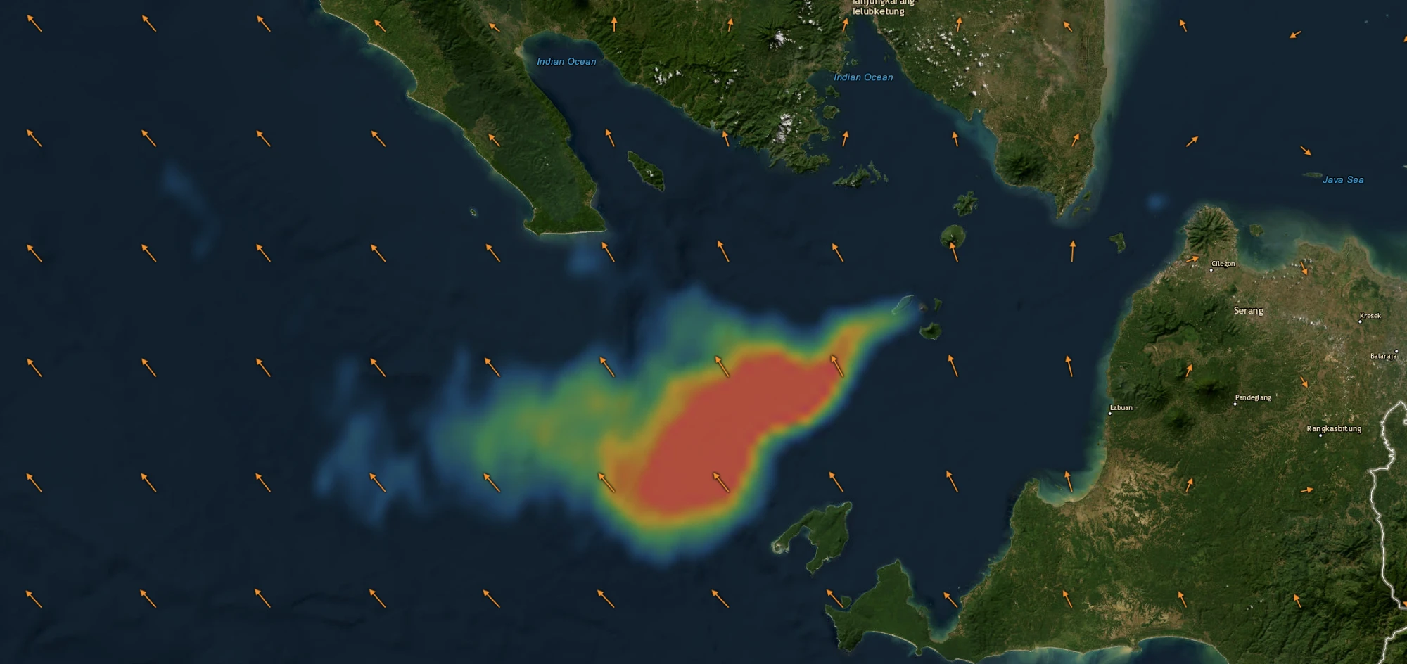
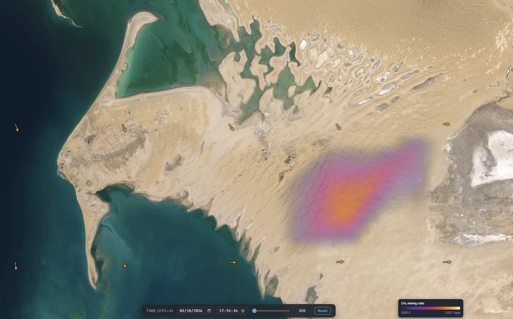
SO2 column density or CH4 (methane) mixing ratio from the Sentinel-5P TROPOMI instrument,
regridded onto a regular lat/lon grid and rendered as its own color ramp — a six-stop heat
ramp (blue through red) for SO2, a distinct violet-to-amber ramp for CH4 so the two never
read as the same thing. NOAA GFS 10 m wind is sampled on a 13×13 grid over the same
footprint and drawn as directional arrows — so concentration and drift direction read as one
picture, for volcanic SO2, refinery and industrial plumes, pipeline/methane sources, or
cross-border pollution events.
How it is fetched
Both sources are queried live for the AOI and date requested — the SO2/CH4 swath via
Copernicus' Data Space Ecosystem (CDSE), the wind field from NOAA's public GFS archive. The
source granule is cached once per scene, shared across jobs, so re-rendering the same
footprint does not re-download it.
What this is, and what it is not. Both layers are real, live-fetched data —
nothing here is synthesized. What it is not: a dispersion or plume-transport model. The wind
arrows show the wind field at the time of the pass, not a forecast of where the gas will be in
six hours — reading that forward is left to you, the same way it would be with the raw sources.
Atmospheric Fusion · SO2 column density + wind vectors, Sunda Strait
Atmospheric Fusion · CH4 mixing ratio + wind vectors, Hazar, Turkmenistan
Public data layers
A growing library of context, not just gas and wind
SO2 fusion is the deepest example — two sources merged into one physically meaningful layer —
but it sits alongside a wider, growing set of public map layers, each toggled straight from
the same Intelligence Layers panel.
Air quality — NO2 (CAMS)
Global nitrogen dioxide forecast from Copernicus' Atmosphere Monitoring Service, updated
every 3 hours — context for industrial activity and urban pollution even on days a
satellite swath does not cross the AOI at all.
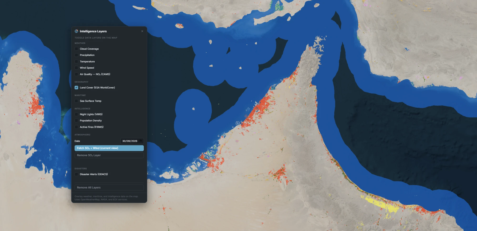
Land cover (ESA WorldCover)
10 m global land classification — forest, cropland, built-up, water and more. The base
layer every other signal on this page reads against: an NDVI drop means something different
over cropland than over forest.
Disaster alerts (GDACS)
Live multi-hazard feed from the UN/European Commission's Global Disaster Alert and
Coordination System — earthquakes, floods, cyclones, volcanoes, severity-scored, each
pinned with a link to the full report.
Orbital conjunctions (SOCRATES)
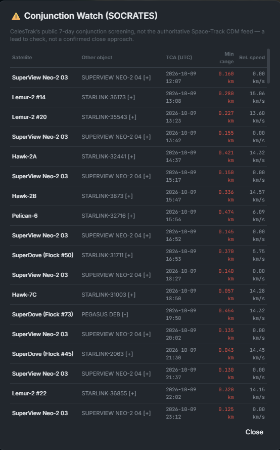
CelesTrak's close-approach screening against the full unclassified catalog, filtered to the
satellites you're already tracking — a lead to verify, not a confirmed collision warning,
refreshed several times a day.
News events (GDELT)
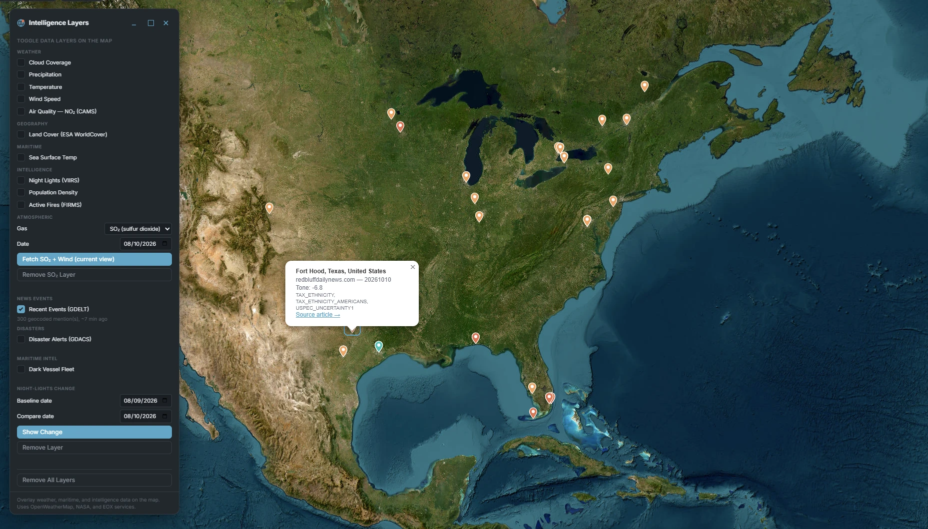
Global news events from GDELT's Global Knowledge Graph, geocoded to city level and colored
by tone, refreshed roughly every 15 minutes — open-press context next to an AOI, not a
confirmed intelligence report.
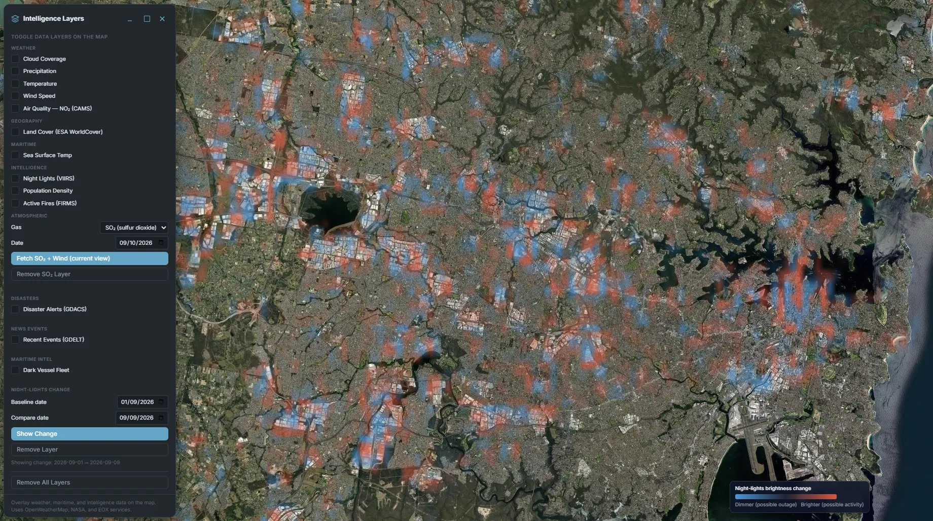
Night-lights change
Diffs NASA's Black Marble VNP46A2 product — calibrated, gap-filled nighttime radiance,
not a rendered tile — between two dates you pick. Dimmer areas flagged as a possible
power outage, brighter ones as possible new activity, cloud- and fill-masked pixel by
pixel.
Every concentration layer carries its own scale. SO2, CH4 and air-quality
overlays show a live color-scale legend on the map itself — the real value range for that
specific job, not a fixed illustrative gradient — and it disappears the moment the layer is
removed.
Land Cover (ESA WorldCover) · Dubai & Abu Dhabi coastline, 10 m classification
Night-Lights Change · calibrated VIIRS (VNP46A2) brightness diff, Sydney, Australia
News Events (GDELT) · geocoded mentions, eastern North America
Orbital Conjunctions (SOCRATES) · 7-day close-approach screening
Correlation & tracking
Six ways SatView reasons about what it already has
No new sensor, no new provider — these cross-reference detections, orbital data and tasking
history that SatView already collects.
AIS correlation & dark-vessel fleet
A ship detection is checked against real AIS broadcast positions within 3 km and
±30 minutes. A match narrows down which vessel it likely is; a track seen at least
twice with no AIS match at all is surfaced as a dark-vessel fleet candidate — fused from AIS
correlation and recurring-entity tracking, a deliberately stricter bar than a single
unmatched sighting, which can just as easily be an AIS coverage gap. AIS history only goes
back as far as SatView has been watching an area — never backfilled.
Recurring entities
Vehicle, ship and aircraft detections are clustered by position (150 m) across repeated
passes. One sighting is just that; two or more at the same spot is surfaced as recurring
activity worth watching over time.
TLE maneuver watch
Every TLE update is compared against the satellite's previous one. A mean-motion jump past
0.005 rev/day, or an inclination change past 0.05°, is logged as a maneuver candidate —
a lead to verify, not a confirmed burn.
Reverse tasking
Give SatView an AOI and it answers a different question: which satellites, across the full
500+ catalog, will pass over it in the next few days — not just the ones you already
selected. A quick way to know who else might be watching the same ground.
Archive vs. new
Before a fresh tasking order goes out, SatView checks the last 30 days of archive across
your connected providers for the same footprint and cloud constraint. A hit surfaces as a
pre-filled shortcut into catalog search — archive imagery typically runs 30-50% cheaper than
tasking, a sector rule of thumb SatView surfaces rather than a quoted price.
Confidence, decomposed
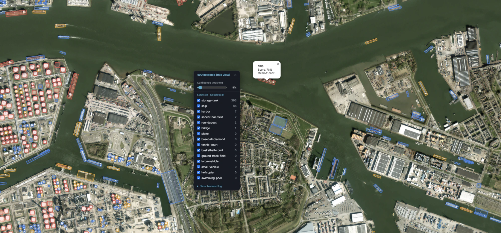
A detection's popup does not collapse everything into one invented percentage. It shows the
model's own detection score, an AIS-correlation confidence tier where it applies, and a
recurrence count — three real signals, kept separate.
Why these stay separate. None of this is calibrated uncertainty quantification —
no conformal intervals, no regional calibration. Each signal is exactly what it says: a real
distance, a real count, a real threshold crossed. Where SatView is not sure, it says so instead
of rounding up to a single confident-looking number.
Detection popup · model score and inference method shown per object
Not every signal is a detection
SatView's safety-simulation suite models physical risk the same discipline as these layers model signals — grounded in real standards, drawn on the actual site.